Motivation
Variational principles provide insight into many physical phenomena: mechanics blossomed with the description of an action functional, such that motion is described by a principle of least action. Many fields including materials science, optics, control theory, image analysis and machine learning have benefited from recasting questions in terms of an appropriate “energy functional,” and exploring its optimizers or equilibrium states.
In general limits of sequences, and as a direct result minimizers of optimization problems, may not exist. This has been a common theme in mathematics since the time of the Babylonian mathematicians Pythagoras and rational or continued fractions approximations to . For a fun discussion of continued fractions see 1. Unfortunately our sequence “runs out of the space.” Or similarly, consider the sequence of smooth functions
The “limit” is well known to be the “-function,” properly interpreted as a distribution on the set of smooth functions or alternatively as a measure. Similarly, minima of variational principles may introduce irregularities, the study of which can be a delicate subject 2.
Throughout the discussion, we will be considering very general problems of the form:
The Direct Method
Hilbert introduced a set of criterion under which minimizers to the problem above are guaranteed: The Direct Method.
Let be a minimizing sequence, i.e.
Then the direct method can be described simply as selecting an appropriate topology satisfying the balance
- is sufficiently coarse to ensure is compact,
- is sufficiently fine to ensure is lower semi-continuous.
Under these conditions, proof of existence of a minimizer becomes relatively simple. Let be a minimizing sequence. In the topology this sequence is (sequentially) compact. Perhaps after selecting an appropriate subsequence, let .
Then, by lower semicontinuity of :
and is a minimizer of . Uniqueness is clearly not guaranteed.
Now suppose that our minimization problem has more structure. That it can be represented as an integral:
The following theorem tells us that convexity is really the key to applying the direct method, and the lack of convexity will result in potential difficulties finding solutions 3.
Theorem
Let be lower semicontinuous, and . Then the mapping
is weakly sequentially lower semicontinuous if and only if is convex.
Nonconvexity and oscillations
Example (Bolza, Young)
Consider the famous Bolza-Young problem:
over the collection of admissable functions
Let . Clearly . In fact, it isn’t too tricky to see that . Consider
periodically extended to . Let . This sawtooth function, with increasingly many teeth of decreasing height satisfying and point-wise for all . However, clearly is not a minimizer.
This fine-scale, oscillatory behavior is a direct consequence of the nonconvexity of the energy. The two “low energy states”: and allow for mixing of the two states and lowering the overall energy as a result. Not only is this mathematically interesting, but physically nonconvex problems are important. My first experience with these ideas, and ultimately what hooked me, were examples from thermodynamics.
Example (Phase mixtures)
Consider the free energy of two different material phases, as a function of mole fraction:
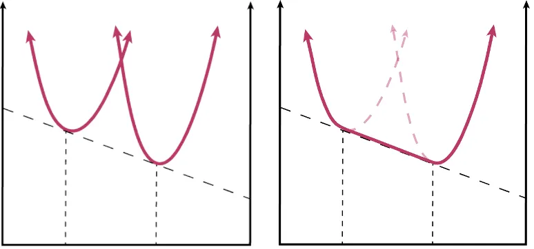
Schematic of the Gibbs energy for two different phases as a function of mole-fraction.
Suppose you have constrained the mole-fraction to be 0.5. Then a pure phase, in either case, will have higher energy than the mixing of two phases (with fractions given by the common tangent line). Mixing to lower the energy can be seen as a “regularization” process in which the observed energy is the convexification of the two energies.
In the absence of surface energy, oscillations would equally well be a minimizer of the Gibbs energy for a mixture, provided that the overall mole-fraction constraint is satisfied.
Example (Phase mixtures, distributions)
Consider the free energy of two different material phases, as a function of mole fraction:
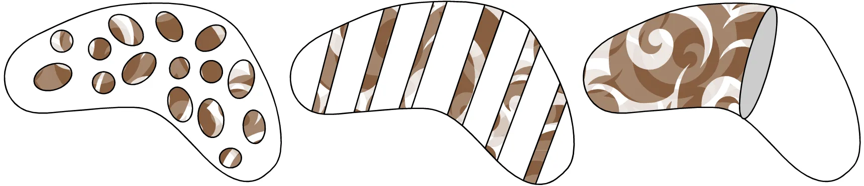
Three equivalent distributions of phase in the lack of surface energy case.
Nonconvex energies exist and oscillations inevitably occur. Young measures represent a concise tool for organizing the information about the oscillatory behavior of minimizing sequences.
Relaxation
Suppose that we’re faced with an optimization problem for which the direct method, or any other method we have tried, which guarantees the existence of a minimizer fails. One thing we can do is relax the problem, i.e., consider an alternative problem for which existence can be shown. However, if this alternative, relaxed problem is too different from the true problem, the solution to the relaxed problem will not tell us anything about our original problem.
I like to think of the process of relaxation as two distinct steps:
- Enlarge the admissable set,
- Reformulate the energy
We can enlarge the admissable set, but not by too much! To this end, it’s often appropriate to ensure that is dense in . Similarly if we adjust the energy too much, then certainly solutions may exist, but the new problem may not provide us with any insight into our true goal, . The new energy must be less than the original, but not substantially so. All of this is very vague; I apologize.
Pedregal describes an general approach to relaxation 4 which should be familiar to most readers.
Choose a collection of functionals, .
- Enlarge the space of admissable objects by completion with respect to this set of functionals.
By this, I mean consider sequences . These two sequences are equivalent if and only if for all . This is much like completing the rational numbers and arriving at or completing a metric space via Cauchy sequences.
- Extend each of the functions to by continuity
where is any representative of .
- Define the topology on as the weak-topology relative to the collection :
Within this framework, we can define the relaxed problem:
Within this framework for relaxation we are guaranteed that we haven’t enlarged the admissable set too much. Density is free. Moreover by continuously extending our functions, the relaxed function approximates our original problem nicely. Moreover, a solution exists. We simply added it as a object, i.e. a limit of a minimizing sequence.
So, if this framework always provides us with a relaxed problem that isn’t relaxed too much, and guarantees the existence of as solution, how is that all of our problems aren’t solved? Well, we need to find a perspective or representation that allows us to handle the limit objects. In many cases, for instance integral optimization, Young measures can be a useful representation. Herein lies the power to this very abstract concept and its application to real-world problems.
References
Footnotes
-
Erik Davis, An introduction to continued fractions. ↩
-
Giuseppe Mingione, Regularity of minima: an invitation to the dark side of the calculus of variations, (2006). ↩
-
Fonseca and Leoni, Modern methods in the calculus of variations, Springer (2007). ↩
-
Pedregal, Optimization, relaxation and Young measures, AMS, (1999). ↩